Selecting or masking a spatial area from a gridded dataset

The select_spatial function is used to select or mask a spatial area from a gridded dataset based on some bounding geometry (e.g. a polygon from a shapefile).

The bounding geometry provided does not need to be in the same coordinate reference system as the gridded dataset; this function will handle necessary conversions.

This function is a thin wrapper around rioxarray’s clip function, and kwargs for that function can be passed through.

import geopandas as gpd 
import ecodata as eco 
import xarray as xr
import hvplot.xarray  # noqa
import hvplot.pandas
import spatialpandas as spd
from pyproj.crs import CRS

Example: Selecting MODIS data within the Y2Y boundary

# Y2Y region boundary 
y2yfile = eco.get_path('y2y_region_priority_areas_2013.gdb')
y2y = gpd.read_file(y2yfile)

Note that this shapefile is not in the same coordinate reference system as the gridded data products. The select_spatial function will handle the conversion to a consistent coordinate system.

y2y.crs

<Derived Projected CRS: PROJCS["WGS_1984_Albers",GEOGCS["WGS 84",DATUM["WG ...>
Name: WGS_1984_Albers
Axis Info [cartesian]:
- [east]: Easting (metre)
- [north]: Northing (metre)
Area of Use:
- undefined
Coordinate Operation:
- name: unnamed
- method: Albers Equal Area
Datum: World Geodetic System 1984
- Ellipsoid: WGS 84
- Prime Meridian: Greenwich

# MODIS NDVI data 
filein = eco.get_path("MOD13A1.006_500m_aid0001_all.nc")
ds = xr.load_dataset(filein)
ds

<xarray.Dataset>
Dimensions:                   (time: 208, lat: 1137, lon: 992)
Coordinates:
  * time                      (time) object 2000-02-18 00:00:00 ... 2009-02-1...
  * lat                       (lat) float64 57.34 57.34 57.33 ... 52.61 52.61
  * lon                       (lon) float64 -123.9 -123.9 ... -119.8 -119.8
Data variables:
    crs                       int8 -127
    _500m_16_days_NDVI        (time, lat, lon) float32 0.3663 0.3146 ... -0.0013
    _500m_16_days_VI_Quality  (time, lat, lon) float64 2.076e+04 ... 1.845e+04
Attributes:
    title:        MOD13A1.006 for aid0001
    Conventions:  CF-1.6
    institution:  Land Processes Distributed Active Archive Center (LP DAAC)
    source:       AppEEARS v3.4
    references:   See README.md
    history:      See README.md

xarray.Dataset

• Dimensions:
  • time: 208
  • lat: 1137
  • lon: 992
• Coordinates: (3)
  • time
    (time)
    object
    2000-02-18 00:00:00 ... 2009-02-...

    standard_name :

    time

    axis :

    T

    array([cftime.DatetimeJulian(2000, 2, 18, 0, 0, 0, 0, has_year_zero=False),
           cftime.DatetimeJulian(2000, 3, 5, 0, 0, 0, 0, has_year_zero=False),
           cftime.DatetimeJulian(2000, 3, 21, 0, 0, 0, 0, has_year_zero=False),
           ...,
           cftime.DatetimeJulian(2009, 1, 17, 0, 0, 0, 0, has_year_zero=False),
           cftime.DatetimeJulian(2009, 2, 2, 0, 0, 0, 0, has_year_zero=False),
           cftime.DatetimeJulian(2009, 2, 18, 0, 0, 0, 0, has_year_zero=False)],
          dtype=object)

  • lat
    (lat)
    float64
    57.34 57.34 57.33 ... 52.61 52.61

    standard_name :

    latitude

    units :

    degrees_north

    _CoordinateAxisType :

    GeoY

    axis :

    Y

    array([57.339583, 57.335417, 57.33125 , ..., 52.614583, 52.610417, 52.60625 ])

  • lon
    (lon)
    float64
    -123.9 -123.9 ... -119.8 -119.8

    standard_name :

    longitude

    units :

    degrees_east

    _CoordinateAxisType :

    GeoX

    axis :

    X

    array([-123.914583, -123.910417, -123.90625 , ..., -119.79375 , -119.789583,
           -119.785417])

• Data variables: (3)
  • crs
    ()
    int8
    -127

    grid_mapping_name :

    latitude_longitude

    _CoordinateAxisTypes :

    GeoX GeoY

    spatial_ref :

    GEOGCS["unknown",DATUM["WGS_1984",SPHEROID["WGS 84",6378137,298.257223563,AUTHORITY["EPSG","7030"]],AUTHORITY["EPSG","6326"]],PRIMEM["Greenwich",0,AUTHORITY["EPSG","8901"]],UNIT["degree",0.0174532925199433,AUTHORITY["EPSG","9122"]],AXIS["Longitude",EAST],AXIS["Latitude",NORTH]]

    epsg_code :

    4326

    semi_major_axis :

    6378137

    inverse_flattening :

    298.257223563

    longitude_of_prime_meridian :

    0.0

    array(-127, dtype=int8)

  • _500m_16_days_NDVI
    (time, lat, lon)
    float32
    0.3663 0.3146 ... 0.0029 -0.0013

    grid_mapping :

    crs

    valid_min :

    -2000

    valid_max :

    10000

    long_name :

    500m 16 days NDVI

    units :

    NDVI

    scale_factor_err :

    0.0

    add_offset_err :

    0.0

    calibrated_nt :

    5

    array([[[ 0.3663    ,  0.3146    ,  0.3146    , ...,  0.0537    ,
              0.1391    ,  0.1391    ],
            [ 0.0492    , -0.0173    ,  0.2794    , ...,  0.08679999,
              0.0872    ,  0.0872    ],
            [-0.0887    , -0.0887    ,  0.0103    , ...,  0.0863    ,
              0.0863    ,  0.1236    ],
            ...,
            [ 0.11409999,  0.1846    ,  0.1788    , ...,         nan,
                     nan,         nan],
            [ 0.0903    ,  0.0903    ,  0.2482    , ...,         nan,
                     nan,         nan],
            [ 0.3486    ,  0.33859998,  0.33859998, ...,         nan,
                     nan, -0.0213    ]],
    
           [[ 0.3771    ,  0.4622    ,  0.4622    , ...,  0.0558    ,
              0.12459999,  0.12459999],
            [-0.0452    ,  0.1054    ,  0.0318    , ...,  0.037     ,
              0.06439999,  0.06439999],
            [-0.0214    , -0.0214    ,  0.0153    , ...,  0.0931    ,
              0.0931    ,  0.0834    ],
    ...
            [ 0.15079999,  0.1232    ,  0.4285    , ...,         nan,
                     nan,         nan],
            [ 0.15079999,  0.15079999,  0.4793    , ...,  0.005     ,
             -0.0091    ,         nan],
            [ 0.14729999,  0.2906    ,  0.2906    , ..., -0.0223    ,
             -0.0223    , -0.0238    ]],
    
           [[-0.0051    ,  0.1424    ,  0.1424    , ...,  0.0476    ,
              0.0971    ,  0.0971    ],
            [ 0.0904    ,  0.01      ,  0.01      , ...,  0.0646    ,
              0.0538    ,  0.0538    ],
            [-0.0163    , -0.0163    ,  0.01      , ...,  0.064     ,
              0.064     ,  0.0887    ],
            ...,
            [ 0.1407    ,  0.0611    ,  0.1801    , ..., -0.0025    ,
             -0.0188    , -0.0188    ],
            [ 0.1407    ,  0.1407    ,  0.0985    , ...,  0.0055    ,
              0.0009    , -0.01      ],
            [ 0.0668    ,  0.1016    ,  0.1016    , ...,  0.0029    ,
              0.0029    , -0.0013    ]]], dtype=float32)

  • _500m_16_days_VI_Quality
    (time, lat, lon)
    float64
    2.076e+04 2.255e+04 ... 1.845e+04

    grid_mapping :

    crs

    valid_min :

    0

    valid_max :

    65534

    long_name :

    500m 16 days VI Quality

    units :

    bit field

    Legend :

    Bit Fields Description (Right to Left): [0-1] : MODLAND_QA [2 bit range] 00: VI produced, good quality 01: VI produced, but check other QA 10: Pixel produced, but most probably cloudy 11: Pixel not produced due to other reasons than clouds [2-5] : VI usefulness [4 bit range] 0000: Highest quality 0001: Lower quality 0010..1010: Decreasing quality 1100: Lowest quality 1101: Quality so low that it is not useful 1110: L1B data faulty 1111: Not useful for any other reason/not processed [6-7] : Aerosol quantity [2 bit range] 00: Climatology 01: Low 10: Average 11: High (11) [8] : Adjacent cloud detected; [1 bit range] 1: Yes 0: No [9] : Atmosphere BRDF correction performed [1 bit range] 1: Yes 0: No [10] : Mixed clouds [1 bit range] 1: Yes 0: No [11-13] : Land/Water Flag [3 bit range] 000: Shallow ocean 001: Land (Nothing else but land) 010: Ocean coastlines and lake shorelines 011: Shallow inland water 100: Ephemeral water 101: Deep inland water 110: Moderate or continental ocean 111: Deep ocean [14] : Possible snow/ice [1 bit range] 1: Yes 0: No [15] : Possible shadow [1 bit range] 1: Yes 0: No

    array([[[20757., 22546., 22546., ..., 18449., 18453., 18453.],
            [20498., 20498., 22546., ..., 18453., 18453., 18453.],
            [20498., 20498., 20542., ..., 18449., 18449., 18453.],
            ...,
            [18449., 18445., 18493., ...,    nan,    nan,    nan],
            [18449., 18449., 18449., ...,    nan,    nan,    nan],
            [18449., 18445., 18445., ...,    nan,    nan,  2058.]],
    
           [[22546., 22546., 22546., ..., 18449., 18453., 18453.],
            [20757., 20757., 22550., ..., 18449., 18449., 18449.],
            [22550., 22550., 20498., ..., 18453., 18453., 18449.],
            ...,
            [18445., 18445., 18445., ..., 18449.,  2058.,  2058.],
            [18705., 18705.,  2110., ..., 18449., 18449., 18449.],
            [18453., 18705., 18705., ..., 18449., 18449., 18449.]],
    
           [[53529., 55577., 55577., ...,  2257., 18449., 18449.],
            [22542., 22542., 37146., ...,  2257.,  2257.,  2257.],
            [53533., 53533., 53533., ...,  2257.,  2257.,  2257.],
            ...,
    ...
            ...,
            [18709., 18454., 18454., ..., 51485., 51485., 51485.],
            [18709., 18709., 18454., ..., 18453., 51485., 18453.],
            [35098., 18454., 18454., ..., 51485., 51485., 18449.]],
    
           [[20757., 20757., 20757., ..., 18449., 18449., 18449.],
            [20498., 22546., 22546., ..., 18449., 18449., 18449.],
            [20502., 20502., 20502., ..., 18449., 18449., 18449.],
            ...,
            [18709., 18450.,  2517., ...,    nan,    nan,    nan],
            [18709., 18709.,  3558., ..., 18449., 18449.,    nan],
            [18450., 18905., 18905., ...,  2322.,  2322., 18449.]],
    
           [[53537., 20761., 20761., ..., 18449., 18449., 18449.],
            [20761., 20501., 20501., ..., 18449., 18449., 18449.],
            [20501., 20501., 20501., ..., 18449., 18449., 18449.],
            ...,
            [18449., 18449., 18449., ..., 18449.,  2062.,  2062.],
            [18449., 18449., 18449., ..., 18449., 18449., 18449.],
            [18449., 18449., 18449., ..., 18449., 18449., 18449.]]])

• Attributes: (6)

  title :

  MOD13A1.006 for aid0001

  Conventions :

  CF-1.6

  institution :

  Land Processes Distributed Active Archive Center (LP DAAC)

  source :

  AppEEARS v3.4

  references :

  See README.md

  history :

  See README.md

# Select MODIS data that falls within the y2y boundary 
ds_subset = eco.select_spatial(ds, boundary=y2y)
ds_subset

<xarray.Dataset>
Dimensions:                   (time: 208, lat: 1137, lon: 992)
Coordinates:
  * time                      (time) object 2000-02-18 00:00:00 ... 2009-02-1...
  * lat                       (lat) float64 57.34 57.34 57.33 ... 52.61 52.61
  * lon                       (lon) float64 -123.9 -123.9 ... -119.8 -119.8
    crs                       int64 0
Data variables:
    _500m_16_days_NDVI        (time, lat, lon) float32 0.3663 0.3146 ... -0.0013
    _500m_16_days_VI_Quality  (time, lat, lon) float64 2.076e+04 ... 1.845e+04
Attributes:
    title:        MOD13A1.006 for aid0001
    Conventions:  CF-1.6
    institution:  Land Processes Distributed Active Archive Center (LP DAAC)
    source:       AppEEARS v3.4
    references:   See README.md
    history:      See README.md

xarray.Dataset

• Dimensions:
  • time: 208
  • lat: 1137
  • lon: 992
• Coordinates: (4)
  • time
    (time)
    object
    2000-02-18 00:00:00 ... 2009-02-...

    standard_name :

    time

    axis :

    T

    array([cftime.DatetimeJulian(2000, 2, 18, 0, 0, 0, 0, has_year_zero=False),
           cftime.DatetimeJulian(2000, 3, 5, 0, 0, 0, 0, has_year_zero=False),
           cftime.DatetimeJulian(2000, 3, 21, 0, 0, 0, 0, has_year_zero=False),
           ...,
           cftime.DatetimeJulian(2009, 1, 17, 0, 0, 0, 0, has_year_zero=False),
           cftime.DatetimeJulian(2009, 2, 2, 0, 0, 0, 0, has_year_zero=False),
           cftime.DatetimeJulian(2009, 2, 18, 0, 0, 0, 0, has_year_zero=False)],
          dtype=object)

  • lat
    (lat)
    float64
    57.34 57.34 57.33 ... 52.61 52.61

    standard_name :

    latitude

    units :

    degrees_north

    _CoordinateAxisType :

    GeoY

    axis :

    Y

    long_name :

    latitude

    array([57.339583, 57.335417, 57.33125 , ..., 52.614583, 52.610417, 52.60625 ])

  • lon
    (lon)
    float64
    -123.9 -123.9 ... -119.8 -119.8

    standard_name :

    longitude

    units :

    degrees_east

    _CoordinateAxisType :

    GeoX

    axis :

    X

    long_name :

    longitude

    array([-123.914583, -123.910417, -123.90625 , ..., -119.79375 , -119.789583,
           -119.785417])

  • crs
    ()
    int64
    0

    crs_wkt :

    GEOGCS["WGS 84",DATUM["WGS_1984",SPHEROID["WGS 84",6378137,298.257223563,AUTHORITY["EPSG","7030"]],AUTHORITY["EPSG","6326"]],PRIMEM["Greenwich",0,AUTHORITY["EPSG","8901"]],UNIT["degree",0.0174532925199433,AUTHORITY["EPSG","9122"]],AXIS["Latitude",NORTH],AXIS["Longitude",EAST],AUTHORITY["EPSG","4326"]]

    semi_major_axis :

    6378137.0

    semi_minor_axis :

    6356752.314245179

    inverse_flattening :

    298.257223563

    reference_ellipsoid_name :

    WGS 84

    longitude_of_prime_meridian :

    0.0

    prime_meridian_name :

    Greenwich

    geographic_crs_name :

    WGS 84

    grid_mapping_name :

    latitude_longitude

    spatial_ref :

    GEOGCS["WGS 84",DATUM["WGS_1984",SPHEROID["WGS 84",6378137,298.257223563,AUTHORITY["EPSG","7030"]],AUTHORITY["EPSG","6326"]],PRIMEM["Greenwich",0,AUTHORITY["EPSG","8901"]],UNIT["degree",0.0174532925199433,AUTHORITY["EPSG","9122"]],AXIS["Latitude",NORTH],AXIS["Longitude",EAST],AUTHORITY["EPSG","4326"]]

    GeoTransform :

    -123.91666665556556 0.004166666666293395 0.0 57.3416666615297 0.0 -0.004166666666293395

    array(0)

• Data variables: (2)
  • _500m_16_days_NDVI
    (time, lat, lon)
    float32
    0.3663 0.3146 ... 0.0029 -0.0013

    grid_mapping :

    crs

    valid_min :

    -2000

    valid_max :

    10000

    long_name :

    500m 16 days NDVI

    units :

    NDVI

    scale_factor_err :

    0.0

    add_offset_err :

    0.0

    calibrated_nt :

    5

    array([[[ 0.3663    ,  0.3146    ,  0.3146    , ...,         nan,
                     nan,         nan],
            [ 0.0492    , -0.0173    ,  0.2794    , ...,         nan,
                     nan,         nan],
            [-0.0887    , -0.0887    ,  0.0103    , ...,         nan,
                     nan,         nan],
            ...,
            [        nan,         nan,         nan, ...,         nan,
                     nan,         nan],
            [        nan,         nan,         nan, ...,         nan,
                     nan,         nan],
            [        nan,         nan,         nan, ...,         nan,
                     nan, -0.0213    ]],
    
           [[ 0.3771    ,  0.4622    ,  0.4622    , ...,         nan,
                     nan,         nan],
            [-0.0452    ,  0.1054    ,  0.0318    , ...,         nan,
                     nan,         nan],
            [-0.0214    , -0.0214    ,  0.0153    , ...,         nan,
                     nan,         nan],
    ...
            [        nan,         nan,         nan, ...,         nan,
                     nan,         nan],
            [        nan,         nan,         nan, ...,  0.005     ,
             -0.0091    ,         nan],
            [        nan,         nan,         nan, ..., -0.0223    ,
             -0.0223    , -0.0238    ]],
    
           [[-0.0051    ,  0.1424    ,  0.1424    , ...,         nan,
                     nan,         nan],
            [ 0.0904    ,  0.01      ,  0.01      , ...,         nan,
                     nan,         nan],
            [-0.0163    , -0.0163    ,  0.01      , ...,         nan,
                     nan,         nan],
            ...,
            [        nan,         nan,         nan, ..., -0.0025    ,
             -0.0188    , -0.0188    ],
            [        nan,         nan,         nan, ...,  0.0055    ,
              0.0009    , -0.01      ],
            [        nan,         nan,         nan, ...,  0.0029    ,
              0.0029    , -0.0013    ]]], dtype=float32)

  • _500m_16_days_VI_Quality
    (time, lat, lon)
    float64
    2.076e+04 2.255e+04 ... 1.845e+04

    grid_mapping :

    crs

    valid_min :

    0

    valid_max :

    65534

    long_name :

    500m 16 days VI Quality

    units :

    bit field

    Legend :

    Bit Fields Description (Right to Left): [0-1] : MODLAND_QA [2 bit range] 00: VI produced, good quality 01: VI produced, but check other QA 10: Pixel produced, but most probably cloudy 11: Pixel not produced due to other reasons than clouds [2-5] : VI usefulness [4 bit range] 0000: Highest quality 0001: Lower quality 0010..1010: Decreasing quality 1100: Lowest quality 1101: Quality so low that it is not useful 1110: L1B data faulty 1111: Not useful for any other reason/not processed [6-7] : Aerosol quantity [2 bit range] 00: Climatology 01: Low 10: Average 11: High (11) [8] : Adjacent cloud detected; [1 bit range] 1: Yes 0: No [9] : Atmosphere BRDF correction performed [1 bit range] 1: Yes 0: No [10] : Mixed clouds [1 bit range] 1: Yes 0: No [11-13] : Land/Water Flag [3 bit range] 000: Shallow ocean 001: Land (Nothing else but land) 010: Ocean coastlines and lake shorelines 011: Shallow inland water 100: Ephemeral water 101: Deep inland water 110: Moderate or continental ocean 111: Deep ocean [14] : Possible snow/ice [1 bit range] 1: Yes 0: No [15] : Possible shadow [1 bit range] 1: Yes 0: No

    array([[[20757., 22546., 22546., ...,    nan,    nan,    nan],
            [20498., 20498., 22546., ...,    nan,    nan,    nan],
            [20498., 20498., 20542., ...,    nan,    nan,    nan],
            ...,
            [   nan,    nan,    nan, ...,    nan,    nan,    nan],
            [   nan,    nan,    nan, ...,    nan,    nan,    nan],
            [   nan,    nan,    nan, ...,    nan,    nan,  2058.]],
    
           [[22546., 22546., 22546., ...,    nan,    nan,    nan],
            [20757., 20757., 22550., ...,    nan,    nan,    nan],
            [22550., 22550., 20498., ...,    nan,    nan,    nan],
            ...,
            [   nan,    nan,    nan, ..., 18449.,  2058.,  2058.],
            [   nan,    nan,    nan, ..., 18449., 18449., 18449.],
            [   nan,    nan,    nan, ..., 18449., 18449., 18449.]],
    
           [[53529., 55577., 55577., ...,    nan,    nan,    nan],
            [22542., 22542., 37146., ...,    nan,    nan,    nan],
            [53533., 53533., 53533., ...,    nan,    nan,    nan],
            ...,
    ...
            ...,
            [   nan,    nan,    nan, ..., 51485., 51485., 51485.],
            [   nan,    nan,    nan, ..., 18453., 51485., 18453.],
            [   nan,    nan,    nan, ..., 51485., 51485., 18449.]],
    
           [[20757., 20757., 20757., ...,    nan,    nan,    nan],
            [20498., 22546., 22546., ...,    nan,    nan,    nan],
            [20502., 20502., 20502., ...,    nan,    nan,    nan],
            ...,
            [   nan,    nan,    nan, ...,    nan,    nan,    nan],
            [   nan,    nan,    nan, ..., 18449., 18449.,    nan],
            [   nan,    nan,    nan, ...,  2322.,  2322., 18449.]],
    
           [[53537., 20761., 20761., ...,    nan,    nan,    nan],
            [20761., 20501., 20501., ...,    nan,    nan,    nan],
            [20501., 20501., 20501., ...,    nan,    nan,    nan],
            ...,
            [   nan,    nan,    nan, ..., 18449.,  2062.,  2062.],
            [   nan,    nan,    nan, ..., 18449., 18449., 18449.],
            [   nan,    nan,    nan, ..., 18449., 18449., 18449.]]])

• Attributes: (6)

  title :

  MOD13A1.006 for aid0001

  Conventions :

  CF-1.6

  institution :

  Land Processes Distributed Active Archive Center (LP DAAC)

  source :

  AppEEARS v3.4

  references :

  See README.md

  history :

  See README.md

# Plot the results with the y2y boundary
y2y_proj = spd.GeoDataFrame(y2y.to_crs(CRS.from_user_input(ds_subset.rio.crs)))
y2y_proj.hvplot(alpha=0.2) * ds_subset.hvplot(x='lon', y='lat', z = '_500m_16_days_NDVI', groupby='time', cmap='Greens') 

# Plot just the spatial subset
ds_subset.hvplot(x='lon', y='lat', z = '_500m_16_days_NDVI', groupby='time', cmap='Greens')

Example: Selecting ECMWF data within the Y2Y boundary

This example uses temperature data from ECMWF

#ECMWF dataset 
filein = eco.get_path("ECMWF_short.nc")
ds = xr.load_dataset(filein)

# Plot the original dataset
ds.hvplot(x='longitude', y='latitude', z = 't2m', groupby='time', cmap='coolwarm')

# Select data within the Y2Y boundary 
ds_subset = eco.select_spatial(ds, boundary=y2y)

# Plot the results 
y2y_proj = spd.GeoDataFrame(y2y.to_crs(CRS.from_user_input(ds_subset.rio.crs)))
y2y_proj.hvplot(alpha=0.2) * ds_subset.hvplot(x='longitude', y='latitude', z = 't2m', groupby='time', cmap='coolwarm') 

Example: Multiple polygons

The select_spatial function will handle cases where the bounding geometry contains multiple polygons.

#ECMWF dataset 
filein = eco.get_path("ECMWF_subset.nc")
ds = xr.load_dataset(filein)

# Plot the original dataset
ds.hvplot(x='longitude', y='latitude', z = 't2m', groupby='time', cmap='coolwarm')

# Example shapefile with multiple polygons 
filein = eco.get_path('combined_poly_overlapping.shp')
shp = gpd.read_file(filein)

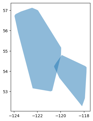
Here, we use a simple example shapefile that contains two polygons:

shp.plot(alpha=0.5)

<AxesSubplot: >

# Select data that falls within the bounding polygons 
ds_subset = eco.select_spatial(ds, boundary=shp)
ds_subset

<xarray.Dataset>
Dimensions:      (longitude: 24, latitude: 19, time: 720)
Coordinates:
  * longitude    (longitude) float32 -123.8 -123.5 -123.2 ... -118.2 -118.0
  * latitude     (latitude) float32 57.0 56.75 56.5 56.25 ... 53.0 52.75 52.5
  * time         (time) datetime64[ns] 2008-06-01 ... 2008-06-30T23:00:00
    spatial_ref  int64 0
Data variables:
    u10          (time, latitude, longitude) float32 nan nan nan ... 1.055 nan
    v10          (time, latitude, longitude) float32 nan nan nan ... 0.2269 nan
    t2m          (time, latitude, longitude) float32 nan nan nan ... 296.2 nan
Attributes:
    Conventions:  CF-1.6
    history:      2022-06-14 00:45:00 GMT by grib_to_netcdf-2.24.3: /opt/ecmw...

xarray.Dataset

• Dimensions:
  • longitude: 24
  • latitude: 19
  • time: 720
• Coordinates: (4)
  • longitude
    (longitude)
    float32
    -123.8 -123.5 ... -118.2 -118.0

    units :

    degrees_east

    long_name :

    longitude

    axis :

    X

    standard_name :

    longitude

    array([-123.75, -123.5 , -123.25, -123.  , -122.75, -122.5 , -122.25, -122.  ,
           -121.75, -121.5 , -121.25, -121.  , -120.75, -120.5 , -120.25, -120.  ,
           -119.75, -119.5 , -119.25, -119.  , -118.75, -118.5 , -118.25, -118.  ],
          dtype=float32)

  • latitude
    (latitude)
    float32
    57.0 56.75 56.5 ... 53.0 52.75 52.5

    units :

    degrees_north

    long_name :

    latitude

    axis :

    Y

    standard_name :

    latitude

    array([57.  , 56.75, 56.5 , 56.25, 56.  , 55.75, 55.5 , 55.25, 55.  , 54.75,
           54.5 , 54.25, 54.  , 53.75, 53.5 , 53.25, 53.  , 52.75, 52.5 ],
          dtype=float32)

  • time
    (time)
    datetime64[ns]
    2008-06-01 ... 2008-06-30T23:00:00

    long_name :

    time

    array(['2008-06-01T00:00:00.000000000', '2008-06-01T01:00:00.000000000',
           '2008-06-01T02:00:00.000000000', ..., '2008-06-30T21:00:00.000000000',
           '2008-06-30T22:00:00.000000000', '2008-06-30T23:00:00.000000000'],
          dtype='datetime64[ns]')

  • spatial_ref
    ()
    int64
    0

    crs_wkt :

    GEOGCS["WGS 84",DATUM["WGS_1984",SPHEROID["WGS 84",6378137,298.257223563,AUTHORITY["EPSG","7030"]],AUTHORITY["EPSG","6326"]],PRIMEM["Greenwich",0,AUTHORITY["EPSG","8901"]],UNIT["degree",0.0174532925199433,AUTHORITY["EPSG","9122"]],AXIS["Latitude",NORTH],AXIS["Longitude",EAST],AUTHORITY["EPSG","4326"]]

    semi_major_axis :

    6378137.0

    semi_minor_axis :

    6356752.314245179

    inverse_flattening :

    298.257223563

    reference_ellipsoid_name :

    WGS 84

    longitude_of_prime_meridian :

    0.0

    prime_meridian_name :

    Greenwich

    geographic_crs_name :

    WGS 84

    grid_mapping_name :

    latitude_longitude

    spatial_ref :

    GEOGCS["WGS 84",DATUM["WGS_1984",SPHEROID["WGS 84",6378137,298.257223563,AUTHORITY["EPSG","7030"]],AUTHORITY["EPSG","6326"]],PRIMEM["Greenwich",0,AUTHORITY["EPSG","8901"]],UNIT["degree",0.0174532925199433,AUTHORITY["EPSG","9122"]],AXIS["Latitude",NORTH],AXIS["Longitude",EAST],AUTHORITY["EPSG","4326"]]

    GeoTransform :

    -123.875 0.25 0.0 57.125 0.0 -0.25

    array(0)

• Data variables: (3)
  • u10
    (time, latitude, longitude)
    float32
    nan nan nan ... nan 1.055 nan

    units :

    m s**-1

    long_name :

    10 metre U wind component

    grid_mapping :

    spatial_ref

    array([[[        nan,         nan,         nan, ...,         nan,
                     nan,         nan],
            [ 2.5565493 ,  2.8422852 ,  1.6306448 , ...,         nan,
                     nan,         nan],
            [ 2.3096414 ,  2.6610868 ,  2.202117  , ...,         nan,
                     nan,         nan],
            ...,
            [        nan,         nan,         nan, ...,  1.4942482 ,
              1.4374993 ,  1.3558605 ],
            [        nan,         nan,         nan, ...,  1.2403712 ,
              1.1975605 ,  0.9088378 ],
            [        nan,         nan,         nan, ...,         nan,
              0.7903619 ,         nan]],
    
           [[        nan,         nan,         nan, ...,         nan,
                     nan,         nan],
            [ 2.446038  ,  2.7735891 ,  1.3867238 , ...,         nan,
                     nan,         nan],
            [ 2.2110775 ,  2.6023467 ,  2.2568748 , ...,         nan,
                     nan,         nan],
    ...
            [        nan,         nan,         nan, ...,  1.2543097 ,
              0.6858243 ,  0.03271329],
            [        nan,         nan,         nan, ...,  1.258292  ,
              0.95762205,  0.92476726],
            [        nan,         nan,         nan, ...,         nan,
              1.7371738 ,         nan]],
    
           [[        nan,         nan,         nan, ...,         nan,
                     nan,         nan],
            [ 1.9352973 ,  2.3046634 ,  1.3827415 , ...,         nan,
                     nan,         nan],
            [ 1.881535  ,  2.2578704 ,  1.5519929 , ...,         nan,
                     nan,         nan],
            ...,
            [        nan,         nan,         nan, ...,  1.0492167 ,
              0.25373554, -0.89816904],
            [        nan,         nan,         nan, ...,  1.3130498 ,
              0.69876695, -0.20025623],
            [        nan,         nan,         nan, ...,         nan,
              1.0551903 ,         nan]]], dtype=float32)

  • v10
    (time, latitude, longitude)
    float32
    nan nan nan ... nan 0.2269 nan

    units :

    m s**-1

    long_name :

    10 metre V wind component

    grid_mapping :

    spatial_ref

    array([[[        nan,         nan,         nan, ...,         nan,
                     nan,         nan],
            [-0.09931576, -0.44483376, -0.27207482, ...,         nan,
                     nan,         nan],
            [ 0.00942075, -0.2680099 , -0.16841936, ...,         nan,
                     nan,         nan],
            ...,
            [        nan,         nan,         nan, ...,  0.6110284 ,
              0.5500546 ,  0.35493863],
            [        nan,         nan,         nan, ...,  0.8325663 ,
              0.79496586,  0.7411057 ],
            [        nan,         nan,         nan, ...,         nan,
              1.1099969 ,         nan]],
    
           [[        nan,         nan,         nan, ...,         nan,
                     nan,         nan],
            [ 0.08258915, -0.29951298, -0.2883345 , ...,         nan,
                     nan,         nan],
            [ 0.17201734, -0.17045188, -0.26902604, ...,         nan,
                     nan,         nan],
    ...
            [        nan,         nan,         nan, ..., -0.3391459 ,
             -0.56474876, -0.53832674],
            [        nan,         nan,         nan, ...,  0.6242393 ,
              0.42302597, -0.2812208 ],
            [        nan,         nan,         nan, ...,         nan,
             -0.14911103,         nan]],
    
           [[        nan,         nan,         nan, ...,         nan,
                     nan,         nan],
            [ 0.03177774,  0.00840449,  0.2929486 , ...,         nan,
                     nan,         nan],
            [-0.08305609,  0.05108607,  0.3844093 , ...,         nan,
                     nan,         nan],
            ...,
            [        nan,         nan,         nan, ...,  0.00129092,
             -0.1653707 ,  0.31225705],
            [        nan,         nan,         nan, ...,  1.0002441 ,
              0.95553005,  0.4291234 ],
            [        nan,         nan,         nan, ...,         nan,
              0.22689378,         nan]]], dtype=float32)

  • t2m
    (time, latitude, longitude)
    float32
    nan nan nan 287.8 ... nan 296.2 nan

    units :

    K

    long_name :

    2 metre temperature

    grid_mapping :

    spatial_ref

    array([[[      nan,       nan,       nan, ...,       nan,       nan,
                   nan],
            [287.9192 , 286.07083, 286.48703, ...,       nan,       nan,
                   nan],
            [287.75778, 286.3921 , 287.52673, ...,       nan,       nan,
                   nan],
            ...,
            [      nan,       nan,       nan, ..., 283.2603 , 284.55322,
             287.43497],
            [      nan,       nan,       nan, ..., 282.71753, 283.55783,
             283.49768],
            [      nan,       nan,       nan, ...,       nan, 283.3774 ,
                   nan]],
    
           [[      nan,       nan,       nan, ...,       nan,       nan,
                   nan],
            [287.89703, 285.8287 , 285.94583, ...,       nan,       nan,
                   nan],
            [287.44287, 285.11185, 285.83505, ...,       nan,       nan,
                   nan],
    ...
            [      nan,       nan,       nan, ..., 296.55652, 296.5296 ,
             296.0612 ],
            [      nan,       nan,       nan, ..., 295.40445, 295.08795,
             295.81906],
            [      nan,       nan,       nan, ...,       nan, 295.3728 ,
                   nan]],
    
           [[      nan,       nan,       nan, ...,       nan,       nan,
                   nan],
            [292.44043, 292.22836, 293.602  , ...,       nan,       nan,
                   nan],
            [293.0861 , 292.8329 , 294.05933, ...,       nan,       nan,
                   nan],
            ...,
            [      nan,       nan,       nan, ..., 296.65463, 296.55652,
             296.20993],
            [      nan,       nan,       nan, ..., 295.8887 , 295.5342 ,
             295.28577],
            [      nan,       nan,       nan, ...,       nan, 296.17197,
                   nan]]], dtype=float32)

• Attributes: (2)

  Conventions :

  CF-1.6

  history :

  2022-06-14 00:45:00 GMT by grib_to_netcdf-2.24.3: /opt/ecmwf/mars-client/bin/grib_to_netcdf -S param -o /cache/data3/adaptor.mars.internal-1655167264.1047153-28011-19-b4a2bb83-8868-486b-bf8e-d7bf035eb998.nc /cache/tmp/b4a2bb83-8868-486b-bf8e-d7bf035eb998-adaptor.mars.internal-1655166317.8944476-28011-26-tmp.grib

# Plot the selected subset
shp_proj = spd.GeoDataFrame(shp.to_crs(CRS.from_user_input(ds_subset.rio.crs)))
ds_subset.hvplot(x='longitude', y='latitude', z = 't2m', groupby='time', cmap='coolwarm') * shp_proj.hvplot(fill_color=None)

Masking a gridded dataset

The selection operation can be inverted (i.e., to do masking rather than selection). In this case, data contained within the bounding geometry will be removed, and data outside the bounding geometry will be selected. Simply pass invert=True to the select_spatial function:

ds_subset = eco.select_spatial(ds, boundary=shp, invert=True)
ds_subset.hvplot(x='longitude', y='latitude', z = 't2m', groupby='time', cmap='coolwarm') * shp_proj.hvplot(fill_color=None)

Additional options

Additional arguments supported by rioxarray’s clip function can also be used. As an example, we can modify the way the edge pixels are handled. By default, only pixels whose center is within the bounding geometry are selected, but we can change this so that all pixels that are touched by the bounding geometry will be selected:

ds_subset1 = eco.select_spatial(ds, boundary=shp)  # Default behavior
ds_subset2 = eco.select_spatial(ds, boundary=shp, all_touched=True)  # Keep all pixels touched by the bounding geometry

ds_subset1.hvplot(x='longitude', y='latitude', z = 't2m', groupby='time', cmap='coolwarm', title='Default edge behavior')* shp_proj.hvplot(fill_color=None) 

ds_subset2.hvplot(x='longitude', y='latitude', z = 't2m', groupby='time', cmap='coolwarm', title='all_touched=True') * shp_proj.hvplot(fill_color=None)

# Example for masking 
ds_subset1 = eco.select_spatial(ds, boundary=shp, invert=True)  # Default behavior
ds_subset2 = eco.select_spatial(ds, boundary=shp, invert=True, all_touched=True)  # Keep all pixels touched by the bounding geometry

ds_subset1.hvplot(x='longitude', y='latitude', z = 't2m', groupby='time', cmap='coolwarm', title='Default edge behavior')* shp_proj.hvplot(fill_color=None) 

ds_subset2.hvplot(x='longitude', y='latitude', z = 't2m', groupby='time', cmap='coolwarm', title='all_touched=True')* shp_proj.hvplot(fill_color=None)