Examples for subsetting the GRIP roads dataset.

These examples use the GRIP global roads dataset, in .gdb format, from https://www.globio.info/download-grip-dataset

Saving the subsetted datasets:

The subsetted dataset can be saved to a new shapefile by specifying an output directory using the outfile argument, this is omitted for these examples.

import ecodata as eco

import geopandas as gpd
import matplotlib.pyplot as plt 

%matplotlib inline

The GRIP global roads dataset was installed as a user dataset using the install_dataset function, and thus the full path to the dataset can be retrieved using the get_path function. If you want your datasets to be accessible this way, you can install them to the package.

If a dataset isn’t installed, you can simply use its filepath to access it.

# Shapefile of GRIP Region 1 dataset
roadsfile = eco.get_path("GRIP4_GlobalRoads.gdb")

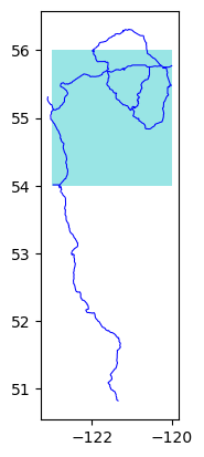
Option 1: Subset the roads dataset using bbox

Small subset, from .gdb global dataset

If you only need to subset a small area without a large number of features, it will be very fast even though it’s subsetting from the entire global dataset:

# Small subset for testing (lat/long bounding box coordinates)
# specify as [long_min, lat_min, long_max, lat_max]
bbox = [-123, 54, -120, 56] 

%%time
subset = eco.subset_data(roadsfile, bbox=bbox)

CPU times: user 13 ms, sys: 7.33 ms, total: 20.3 ms
Wall time: 27.1 ms

The light blue areas in the plots are showing the boundary that was used to make the subset. By default, the function returns all features that intersect with the bounding box, so the subset includes parts of roads extending past the bounding box:

%%time
eco.plot_subset(**subset)

CPU times: user 73.5 ms, sys: 22.3 ms, total: 95.7 ms
Wall time: 44.2 ms

# Deleting each subset between examples for speed tests, so there aren't extra things in memory from the previous tests
del subset   

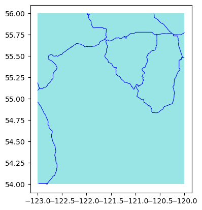
Option to clip features at boundary edge

By default, the function returns all features that intersect with the bounding box, but there is also the option to clip the features at the boundary edge:

%%time
subset = eco.subset_data(roadsfile, bbox=bbox, clip=True)

CPU times: user 25.4 ms, sys: 20.7 ms, total: 46.1 ms
Wall time: 14.1 ms

/Users/jmissik/miniconda3/envs/pmv-dev/lib/python3.9/site-packages/geopandas/tools/clip.py:66: FutureWarning: In a future version, `df.iloc[:, i] = newvals` will attempt to set the values inplace instead of always setting a new array. To retain the old behavior, use either `df[df.columns[i]] = newvals` or, if columns are non-unique, `df.isetitem(i, newvals)`
  clipped.loc[

%%time
eco.plot_subset(**subset)

CPU times: user 87.9 ms, sys: 49.3 ms, total: 137 ms
Wall time: 40.8 ms

del subset   

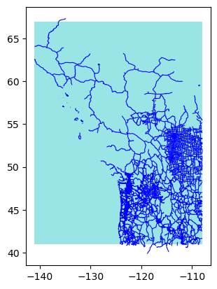
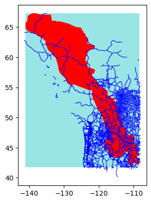
Larger subset, from .gdb global dataset

The requested subset in this example has over 300,000 records, so it takes longer to process and plot:

# Larger subset for testing 
bbox = [-141, 41, -108, 67] 

%%time
subset = eco.subset_data(roadsfile, bbox=bbox)

CPU times: user 6.41 s, sys: 313 ms, total: 6.73 s
Wall time: 6.86 s

# Number of records in the subset
len(subset['subset'])

307280

%%time
eco.plot_subset(**subset)

CPU times: user 20.5 s, sys: 454 ms, total: 20.9 s
Wall time: 20.5 s

del subset   

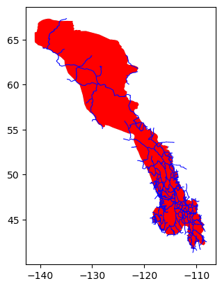
Option 2: Subsetting the roads dataset using bounding geometry from a file

In this case, subsetting using the Y2Y region boundary. The roads dataset and the GIS layer with the Y2Y boundary are in different projections; this is handled.

y2yfile = eco.get_path('y2y_region_priority_areas_2013.gdb')

CRS of the roads dataset and Y2Y dataset:

eco.get_crs(roadsfile)

'epsg:4326'

eco.get_crs(y2yfile)

Failed to auto identify EPSG: 7

'PROJCS["WGS_1984_Albers",GEOGCS["WGS 84",DATUM["WGS_1984",SPHEROID["WGS 84",6378137,298.257223563,AUTHORITY["EPSG","7030"]],AUTHORITY["EPSG","6326"]],PRIMEM["Greenwich",0],UNIT["Degree",0.0174532925199433]],PROJECTION["Albers_Conic_Equal_Area"],PARAMETER["latitude_of_center",42],PARAMETER["longitude_of_center",-120],PARAMETER["standard_parallel_1",42],PARAMETER["standard_parallel_2",68],PARAMETER["false_easting",0],PARAMETER["false_northing",0],UNIT["metre",1,AUTHORITY["EPSG","9001"]],AXIS["Easting",EAST],AXIS["Northing",NORTH]]'

The subset_data function returns a dictionary containing the subsetted data and the subsetting boundary. If a file with bounding geometry is used for subsetting, the bounding geometry will also be returned in this dictionary.

%%time
subset = eco.subset_data(roadsfile, bounding_geom=y2yfile)

Failed to auto identify EPSG: 7

CPU times: user 6.44 s, sys: 184 ms, total: 6.62 s
Wall time: 6.81 s

%%time
eco.plot_subset(**subset)

CPU times: user 19.9 s, sys: 322 ms, total: 20.3 s
Wall time: 19.8 s

del subset   

Using other options for boundary types

Default is to use a rectangular bounding box around the region boundary for subsetting, but there are also options to instead use the actual region boundary, or a convex hull around the region boundary. These options can also be used with a buffer size around the boundary, if you want to get features that are close to the boundary as well.

Here, demonstrating using the actual region boundary to subset. This option can save a lot of time if you have an irreguar boundary shape, and don’t actually need all of the features in the whole bounding box outside the boundary shape:

%%time
subset = eco.subset_data(roadsfile, bounding_geom=y2yfile, boundary_type="mask")

Failed to auto identify EPSG: 7

CPU times: user 1.95 s, sys: 103 ms, total: 2.05 s
Wall time: 2.21 s

%%time
eco.plot_subset(**subset)

CPU times: user 1.91 s, sys: 215 ms, total: 2.12 s
Wall time: 1.68 s

del subset

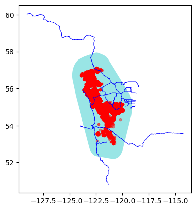
Option 3: Subset the roads dataset using track points

Instead of providing bounding box coordinates or a region boundary for subsetting, you can also provide a csv file with animal track data. A boundary will be drawn around all the track points, with the option for either a rectangular boundary or convex hull.

You can also specify a buffer size with this option.

# Publicly available data from Mountain Caribou in British Columbia study: 
# https://www.movebank.org/cms/webapp?gwt_fragment=page=studies,path=study216040785

track_file = eco.get_path("caribou_data.csv")

Note that the track data in this case includes almost 250,000 points, so processing is a bit slower compared with using a bounding geometry.

If we create a subset using a file with track data, the returned dictionary will also contain the track points. Then, the tracks can also be passed to the plot_subset function.

Here, demonstrating the option to use a convex hull around the track points, with a buffer:

%%time
subset = eco.subset_data(roadsfile, track_points=track_file, boundary_type='convex_hull', buffer=0.2)

CPU times: user 5.68 s, sys: 243 ms, total: 5.92 s
Wall time: 6.06 s

# Number of records in the tracks dataset
len(subset['track_points'])

249450

%%time 
eco.plot_subset(**subset)

CPU times: user 7.34 s, sys: 298 ms, total: 7.64 s
Wall time: 7.12 s